Overview:
-
Two objects that are analysed and that are going to be grouped may have several binary attributes. For example, Fruit Colour is Yellow – Yes, or No if the fruit colour is not yellow. The tree grows in rain forests – Yes, or No tree does not grow in rain forest. In this way the two objects under consideration have many properties one may possess or one may not possess.
-
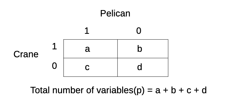
The Boolean properties or traits on two objects will result in the combinations of 11, 10, 01 and 00. Such combinations and their counts are captured in a table called contingency table. The table is also called as an association table.
-
By counting and working on the number of such combinations several dissimilarity metrics come in place. Metrics like the Dice dissimilarity provide more weightage to scenarios when both the attributes evaluate to True. i.e, The binary combination '11' in the contingency table.
-
The Jaccard dissimilarity distance is given by
-
J(i, j) = b + c/a + b + c
-
-
In other words J(i, j) = count(10) + count(01) / count(11) + count(10) + count(01)
Example:
|
Species |
White |
Feeds on Fish |
Flies |
Pouched Beak |
Two legs |
|
Crane |
1 |
1 |
1 |
0 |
1 |
|
Pelican |
1 |
1 |
1 |
1 |
1 |
|
Snow Bear |
1 |
1 |
0 |
0 |
0 |
j(Crane, Pelican) = 0+1/4+1+0
j(Crane, Pelican) = 0.2
The Jaccard dissimilarity between Crane and Pelican is 0.25 meaning the species are different to the extent of 20%.
|
# Example Python program that finds the Jaccard dissimilarity features_crane = [1, 1, 1, 0, 1] jaccard_dissimilarity = dist.jaccard(features_crane, features_pelican) |
Output:
| Jaccard dissimilarity between the species Crane and Pelican: 0.2 |