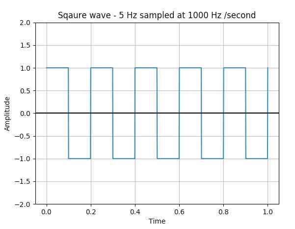
Overview:
- Square waves are period waveforms.
- However, square waves are non-sinusoidal. The transition between the peak values is instantaneous in a square wave.
- The period of the square wave that is starting from a position like zero crossing the time it takes to return to the same position again.
- The period of the square wave is also called the pulse width.
- To draw a square wave using matplotlib, scipy and numpy following details are required
- Frequency of the square wave - Say 10 Hz - That is 10 cycles per second
- The sampling frequency - That is, how many data points with which the square wave is being constructed - higher the data points smoother the square is.
- Square waves have a duty cycle of 50%. That is, the percentage of the waveform that occurs above zero axes is 50% for a square wave.
- By default the signal.square() function of scipy takes a duty value of 0.5.
Example:
|
from scipy import signal import matplotlib.pyplot as plot import numpy as np
# Sampling rate 1000 hz / second t = np.linspace(0, 1, 1000, endpoint=True)
# Plot the square wave signal plot.plot(t, signal.square(2 * np.pi * 5 * t))
# Give a title for the square wave plot plot.title('Square wave - 5 Hz sampled at 1000 Hz /second')
# Give x axis label for the square wave plot plot.xlabel('Time')
# Give y axis label for the square wave plot plot.ylabel('Amplitude')
plot.grid(True, which='both')
# Provide x axis and line color plot.axhline(y=0, color='k')
# Set the max and min values for y axis plot.ylim(-2, 2)
# Display the square wave drawn plot.show() |
Output:
