The skew() function of Pandas library

Overview:

The Skewness is a measure of asymmetry of a probability distribution. Another measure that describes the shape of a distribution is kurtosis. In a normal distribution, the mean divides the curve symmetrically into two equal parts at the median and the value of skewness is zero. When a distribution is asymmetrical the tail of the distribution is skewed to one side - to the right or to the left.

Negatively skewed distribution:

When the value of the skewness is negative, the tail of the distribution is longer towards the left hand side of the curve. The test scores from example 1 are negatively skewed, resulting in a distribution having long tail to the left of the distribution as given in the output below.

Negatively skewed distribution

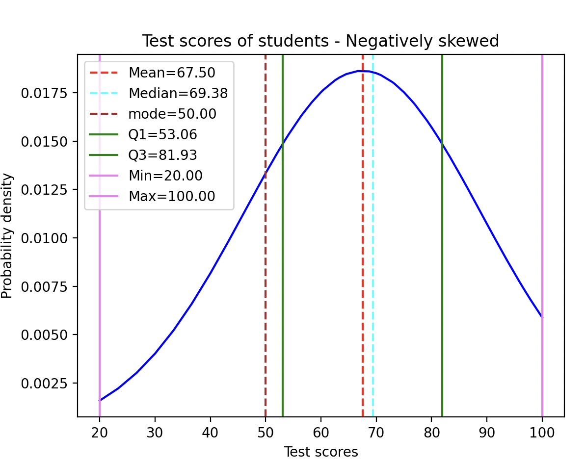
Unlike a symmetrical normal distribution where the mean, median and mode are all equal, these measures are unequal in a negatively skewed distribution. As a result, the mode (most frequent value of the distribution) is the highest, followed by the median (the middle value), and the mean (the average) is the lowest (Mean < Median <Mode). While this is typical of a negatively skewed distribution, in the example below containing test scores the relationship observed is Mode < Mean <median.

The observations loaded into the pandas DataFrame provides a skewness value of -0.416704 for the distribution.

Positively skewed distribution:

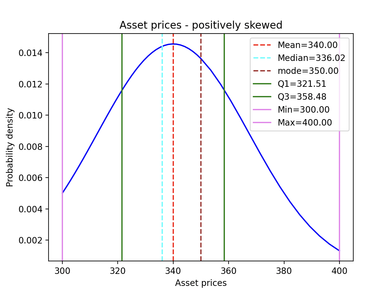
When the value of the skewness is positive, the tail of the distribution is longer towards the right hand side of the curve. The Python example 2 produces a distribution which is skewed to the right side. It plots the price of an asset over time using normal distribution with the help of the matplotlib library and the stats module of scipy. The output from matplotlib is given below:

Positively skewed distribution

The skewness() function in pandas:

The DataFrame class of pandas has a method skew() that computes the skewness of the data present in a given axis of the DataFrame object.
Skewness is computed for each row or each column of the data present in the DataFrame object.

Example 1 - Negatively skewed distribution:

# Example Python program that plots a set of points
# using normal distribution. The distribution obtained
# is skewed to the left
import pandas as pds
import numpy as np
from scipy import stats
import matplotlib.pyplot as plt

# Test scores of 50 students
testScores = [50.0, 52.08, 54.16, 56.25, 58.33,
60.41, 62.5, 64.58, 66.66, 68.75,
70.83, 72.91, 75.0, 77.08, 79.16,
81.25, 83.33, 85.41, 87.50, 89.58,
91.66, 93.75, 95.83, 97.91, 100.0,
20.0, 23.33, 26.66, 30.0, 33.33,
36.66, 40.0, 43.33, 46.66, 50.0,
53.33, 56.66, 60.0, 63.33, 66.66,
70.0, 73.33, 76.66, 80.0, 83.33,
86.66, 90.0, 93.33, 96.66, 100.0]

dataFrame = pds.DataFrame(testScores)
skewVal = dataFrame.skew(axis=0)
print("Skew:")
print(skewVal)

# Find measures of central tendency
# Mean, median, mode and mode count
mean = np.mean(testScores)
median = np.median(testScores)
mode = stats.mode(testScores).mode
modeCount = stats.mode(testScores).count

print("Mean:{:.2f}".format(mean))
print("Median:{:.2f}".format(median))
print("Mode:{:.2f}".format(mode))
print("Mode count:{:.2f}".format(modeCount))

# Find standard deviation
stdDev = np.std(testScores)
print("Standard deviation:{:.2f}".format(stdDev))

# Analysis of quartiles
firstQuartile = mean - (0.67448975 * stdDev)
thirdQuartile = mean + (0.67448975 * stdDev)
min = np.min(testScores)
max = np.max(testScores)

q1Count = ((testScores <= firstQuartile) & (testScores >= min)).sum()
print("Scores in the first quartile:")
print(q1Count)

q2Count = ((testScores <= mean) & (testScores >= firstQuartile)).sum()
print("Scores between first quartile and mean:")
print(q2Count)

q3Count = ((testScores <= thirdQuartile) & (testScores >= mean)).sum()
print("Scores between mean and third quartile:")
print(q3Count)

q4Count = (testScores >= thirdQuartile).sum()
print("Scores beyond third quartile:")
print(q4Count)

# Compute Y values using normal distribution
testScores = np.sort(testScores)
y = stats.norm.pdf(testScores, loc = mean, scale = stdDev)

# Plot the distribution
plt.plot(testScores, y, color = 'blue')
plt.axvline(mean, color='red', linestyle='--', label=f'Mean={mean:.2f}')
plt.axvline(median, color='cyan', linestyle='--', label=f'Median={median:.2f}')
plt.axvline(mode, color='brown', linestyle='--', label=f'mode={mode:.2f}')
plt.axvline(firstQuartile, color='green', linestyle='solid', label=f'Q1={firstQuartile:.2f}')
plt.axvline(thirdQuartile, color='green', linestyle='solid', label=f'Q3={thirdQuartile:.2f}')
plt.axvline(min, color='violet', linestyle='solid', label=f'Min={min:.2f}')
plt.axvline(max, color='violet', linestyle='solid', label=f'Max={max:.2f}')

# Give a title
plt.title('Test scores of students - Negatively skewed')
plt.xlabel('Test scores')
plt.ylabel('Probability density')

# Display the plot
plt.legend()
plt.show()

Output:

Skew:
0 -0.416704
dtype: float64
Mean:67.50
Median:69.38
Mode:50.00
Mode count:2.00
Standard deviation:21.40
Scores in the first quartile:
12
Scores between first quartile and mean:
12
Scores between mean and third quartile:
11
Scores beyond third quartile:
15

Example 2:

# Example Python program that plots a set of points
# using normal distribution. The distribution obtained
# is skewed to the right.
import pandas as pds
import numpy as np
from scipy import stats
import matplotlib.pyplot as plt

assetPrices = [300.0, 301.47, 302.94, 304.41, 305.88,
307.35, 308.82, 310.29, 311.76, 313.23,
314.70, 316.17, 317.64, 319.11, 320.58,
322.05, 323.52, 325.00, 326.47, 327.94,
329.41, 330.88, 332.35, 333.82, 335.29,
336.76, 338.23, 339.70, 341.17, 342.64,
344.11, 345.58, 347.05, 348.52, 350.0,
350.0, 353.57, 357.14, 360.71, 364.28,
367.85, 371.42, 375.0, 378.57, 382.14,
385.71, 389.28, 392.85, 396.42, 400.0]

# Find the value of skewness
df = pds.DataFrame(assetPrices)
skewValue = df.skew(axis=0)
print("Skew")
print(skewValue)

# Find measures of central tendency
# Mean, median, mode and mode count
meanValue = np.mean(assetPrices)
medianValue = np.median(assetPrices)
modeValue = stats.mode(assetPrices).mode
modeCount = stats.mode(assetPrices).count

print("Mean:{:.2f}".format(meanValue))
print("Median:{:.2f}".format(medianValue))
print("Mode:{:.2f}".format(modeValue))
print("Mode count:{:.2f}".format(modeCount))

# Find standard deviation
sigma = np.std(assetPrices)
print("Standard deviation:{:.2f}".format(sigma))

# Analysis of quartiles
quartileOne = meanValue - (0.67448975 * sigma)
quartileThree = meanValue + (0.67448975 * sigma)
min = np.min(assetPrices)
max = np.max(assetPrices)

q1Frequency = ((assetPrices <= quartileOne) & (assetPrices >= min)).sum()
print("Prices in the first quartile:")
print(q1Frequency)

q2Frequency = ((assetPrices <= meanValue) & (assetPrices >= quartileOne)).sum()
print("Prices between first quartile and mean:")
print(q2Frequency)

q3Frequency = ((assetPrices <= quartileThree) & (assetPrices >= meanValue)).sum()
print("Prices between mean and third quartile:")
print(q3Frequency)

q4Frequency = (assetPrices >= quartileThree).sum()
print("Prices beyond third quartile:")
print(q4Frequency)

# Compute Y values using normal distribution
assetPrices = np.sort(assetPrices)
pd = stats.norm.pdf(assetPrices, loc = meanValue, scale = sigma)

# Plot the distribution
plt.plot(assetPrices, pd, color = 'blue')
plt.axvline(meanValue, color='red', linestyle='--', label=f'Mean={meanValue:.2f}')
plt.axvline(medianValue, color='cyan', linestyle='--', label=f'Median={medianValue:.2f}')
plt.axvline(modeValue, color='brown', linestyle='--', label=f'mode={modeValue:.2f}')
plt.axvline(quartileOne, color='green', linestyle='solid', label=f'Q1={quartileOne:.2f}')
plt.axvline(quartileThree, color='green', linestyle='solid', label=f'Q3={quartileThree:.2f}')
plt.axvline(min, color='violet', linestyle='solid', label=f'Min={min:.2f}')
plt.axvline(max, color='violet', linestyle='solid', label=f'Max={max:.2f}')

# Give a title
plt.title('Asset prices - positively skewed')
plt.xlabel('Asset prices')
plt.ylabel('Probability density')

# Display the plot
plt.legend()
plt.show()

Output:

Skew
0 0.553983
dtype: float64
Mean:340.00
Median:336.02
Mode:350.00
Mode count:2.00
Standard deviation:27.40
Prices in the first quartile:
15
Prices between first quartile and mean:
13
Prices between mean and third quartile:
10
Prices beyond third quartile:
12

Example 3:

import pandas as pd

dataVal = [(10,20,30,40,50,60,70),

(10,10,40,40,50,60,70),

(10,20,30,50,50,60,80)]

dataFrame = pd.DataFrame(data=dataVal);

skewValue = dataFrame.skew(axis=1)

print("DataFrame:")

print(dataFrame)

print("Skew:")

print(skewValue)

Output:

DataFrame:

0 1 2 3 4 5 6

0 10 20 30 40 50 60 70

1 10 10 40 40 50 60 70

2 10 20 30 50 50 60 80

Skew:

0 0.000000

1 -0.340998

2 0.121467

dtype: float64

A skewness value of 0 in the output denotes a symmetrical distribution of values in row 1.
A negative skewness value in the output indicates an asymmetry in the distribution corresponding to row 2 and the tail is larger towards the left hand side of the distribution.
A positive skewness value in the output indicates an asymmetry in the distribution corresponding to row 3 and the tail is larger towards the right hand side of the distribution.